NumPy Evaluation

Comprehensive NumPy evaluation metrics for NeuralForecast including MAE, MSE, MAPE, MASE, and probabilistic losses for time series forecast accuracy.

The most important train signal is the forecast error, which is the difference between the observed value $y_{\tau}$ and the prediction $\hat{y}_{\tau}$, at time $y_{\tau}$:

$e_{\tau} = y_{\tau}-\hat{y}_{\tau} \qquad \qquad \tau \in \{t+1,\dots,t+H \}$

The train loss summarizes the forecast errors in different evaluation metrics.

1. Scale-dependent Errors

These metrics are on the same scale as the data.

Mean Absolute Error

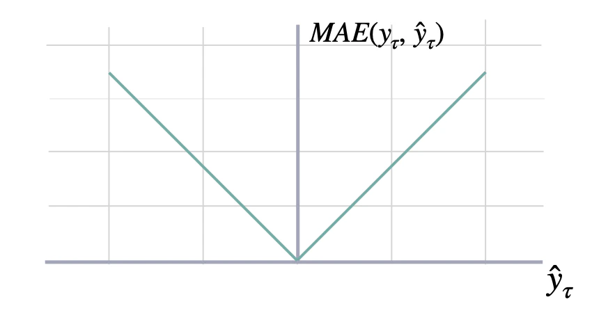
mae

mae(y, y_hat, weights=None, axis=None)

Mean Absolute Error

Calculates Mean Absolute Error between y and y_hat. MAE measures the relative prediction accuracy of a forecasting method by calculating the deviation of the prediction and the true value at a given time and averages these devations over the length of the series.

$$\mathrm{MAE}(\mathbf{y}_{\tau}, \mathbf{\hat{y}}_{\tau}) = \frac{1}{H} \sum^{t+H}_{\tau=t+1} |y_{\tau} - \hat{y}_{\tau}|$$

Parameters:

Name	Type	Description	Default
y	ndarray	Actual values.	required
y_hat	ndarray	Predicted values.	required
mask	ndarray	Specifies date stamps per serie to consider in loss. Defaults to None.	required

Returns:

Name	Type	Description
float	Union[float, ndarray]	MAE.

Mean Squared Error

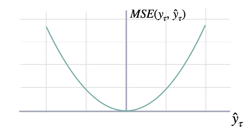
mse

mse(y, y_hat, weights=None, axis=None)

Mean Squared Error

Calculates Mean Squared Error between y and y_hat. MSE measures the relative prediction accuracy of a forecasting method by calculating the squared deviation of the prediction and the true value at a given time, and averages these devations over the length of the series.

$$\mathrm{MSE}(\mathbf{y}_{\tau}, \mathbf{\hat{y}}_{\tau}) = \frac{1}{H} \sum^{t+H}_{\tau=t+1} (y_{\tau} - \hat{y}_{\tau})^{2}$$

Parameters:

Name	Type	Description	Default
y	ndarray	Actual values.	required
y_hat	ndarray	Predicted values.	required
mask	ndarray	Specifies date stamps per serie to consider in loss. Defaults to None.	required

Returns:

Name	Type	Description
float	Union[float, ndarray]	MSE.

Root Mean Squared Error

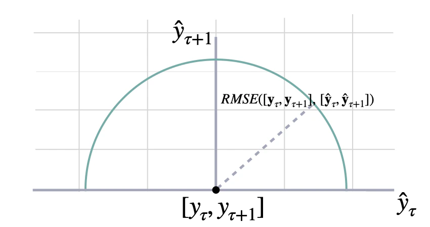
rmse

rmse(y, y_hat, weights=None, axis=None)

Root Mean Squared Error

Calculates Root Mean Squared Error between y and y_hat. RMSE measures the relative prediction accuracy of a forecasting method by calculating the squared deviation of the prediction and the observed value at a given time and averages these devations over the length of the series. Finally the RMSE will be in the same scale as the original time series so its comparison with other series is possible only if they share a common scale. RMSE has a direct connection to the L2 norm.

$$\mathrm{RMSE}(\mathbf{y}_{\tau}, \mathbf{\hat{y}}_{\tau}) = \sqrt{\frac{1}{H} \sum^{t+H}_{\tau=t+1} (y_{\tau} - \hat{y}_{\tau})^{2}}$$

Parameters:

Name	Type	Description	Default
y	ndarray	Actual values.	required
y_hat	ndarray	Predicted values.	required
mask	ndarray	Specifies date stamps per serie to consider in loss. Defaults to None.	required

Returns:

Name	Type	Description
float	Union[float, ndarray]	RMSE.

2. Percentage errors

These metrics are unit-free, suitable for comparisons across series.

Mean Absolute Percentage Error

mape

mape(y, y_hat, weights=None, axis=None)

Mean Absolute Percentage Error

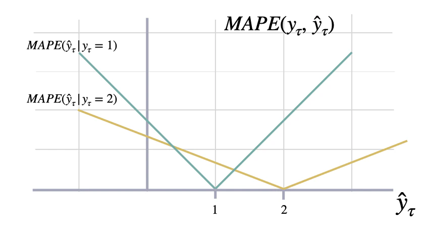
Calculates Mean Absolute Percentage Error between y and y_hat. MAPE measures the relative prediction accuracy of a forecasting method by calculating the percentual deviation of the prediction and the observed value at a given time and averages these devations over the length of the series. The closer to zero an observed value is, the higher penalty MAPE loss assigns to the corresponding error.

$$\mathrm{MAPE}(\mathbf{y}_{\tau}, \mathbf{\hat{y}}_{\tau}) = \frac{1}{H} \sum^{t+H}_{\tau=t+1} \frac{|y_{\tau}-\hat{y}_{\tau}|}{|y_{\tau}|}$$

Parameters:

Name	Type	Description	Default
y	ndarray	Actual values.	required
y_hat	ndarray	Predicted values.	required
mask	ndarray	Specifies date stamps per serie to consider in loss. Defaults to None.	required

Returns:

Name	Type	Description
float	Union[float, ndarray]	MAPE.

SMAPE

smape

smape(y, y_hat, weights=None, axis=None)

Symmetric Mean Absolute Percentage Error

Calculates Symmetric Mean Absolute Percentage Error between y and y_hat. SMAPE measures the relative prediction accuracy of a forecasting method by calculating the relative deviation of the prediction and the observed value scaled by the sum of the absolute values for the prediction and observed value at a given time, then averages these devations over the length of the series. This allows the SMAPE to have bounds between 0% and 200% which is desirable compared to normal MAPE that may be undetermined when the target is zero.

$$\mathrm{sMAPE}_{2}(\mathbf{y}_{\tau}, \mathbf{\hat{y}}_{\tau}) = \frac{1}{H} \sum^{t+H}_{\tau=t+1} \frac{|y_{\tau}-\hat{y}_{\tau}|}{|y_{\tau}|+|\hat{y}_{\tau}|}$$

Parameters:

Name	Type	Description	Default
y	ndarray	Actual values.	required
y_hat	ndarray	Predicted values.	required
mask	ndarray	Specifies date stamps per serie to consider in loss. Defaults to None.	required

Returns:

Name	Type	Description
float	Union[float, ndarray]	SMAPE.

3. Scale-independent Errors

These metrics measure the relative improvements versus baselines.

Mean Absolute Scaled Error

mase

mase(y, y_hat, y_train, seasonality, weights=None, axis=None)

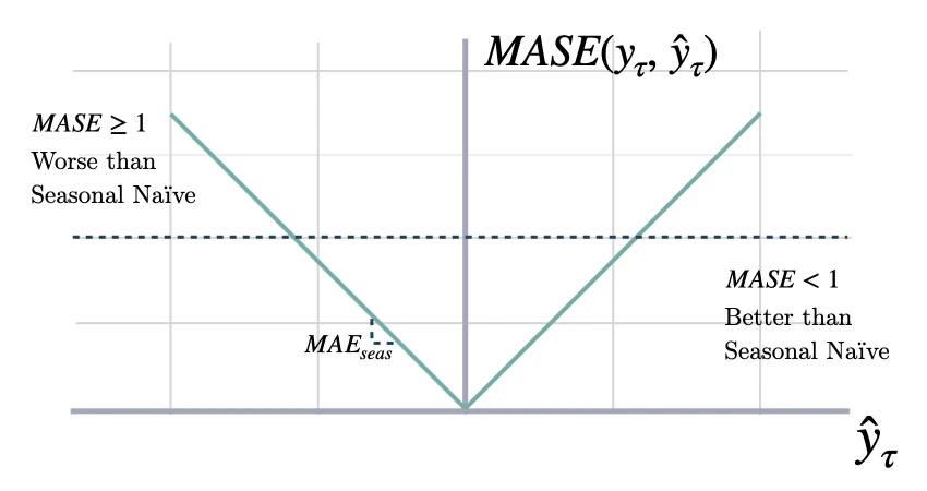
Mean Absolute Scaled Error Calculates the Mean Absolute Scaled Error between y and y_hat. MASE measures the relative prediction accuracy of a forecasting method by comparinng the mean absolute errors of the prediction and the observed value against the mean absolute errors of the seasonal naive model. The MASE partially composed the Overall Weighted Average (OWA), used in the M4 Competition.

$$\mathrm{MASE}(\mathbf{y}_{\tau}, \mathbf{\hat{y}}_{\tau}, \mathbf{\hat{y}}^{season}_{\tau}) = \frac{1}{H} \sum^{t+H}_{\tau=t+1} \frac{|y_{\tau}-\hat{y}_{\tau}|}{\mathrm{MAE}(\mathbf{y}_{\tau}, \mathbf{\hat{y}}^{season}_{\tau})}$$

Parameters:

Name	Type	Description	Default
y	ndarray	Actual values.	required
y_hat	ndarray	Predicted values.	required
y_insample	ndarray	Actual insample Seasonal Naive predictions.	required
seasonality	int	Main frequency of the time series; Hourly 24, Daily 7, Weekly 52, Monthly 12, Quarterly 4, Yearly 1.	required
mask	ndarray	Specifies date stamps per serie to consider in loss. Defaults to None.	required

Returns:

Name	Type	Description
float	Union[float, ndarray]	MASE.

Relative Mean Absolute Error

rmae

rmae(y, y_hat1, y_hat2, weights=None, axis=None)

RMAE

Calculates Relative Mean Absolute Error (RMAE) between two sets of forecasts (from two different forecasting methods). A number smaller than one implies that the forecast in the numerator is better than the forecast in the denominator.

$$\mathrm{rMAE}(\mathbf{y}_{\tau}, \mathbf{\hat{y}}_{\tau}, \mathbf{\hat{y}}^{base}_{\tau}) = \frac{1}{H} \sum^{t+H}_{\tau=t+1} \frac{|y_{\tau}-\hat{y}_{\tau}|}{\mathrm{MAE}(\mathbf{y}_{\tau}, \mathbf{\hat{y}}^{base}_{\tau})}$$

Parameters:

Name	Type	Description	Default
y	ndarray	observed values.	required
y_hat1	ndarray	Predicted values of first model.	required
y_hat2	ndarray	Predicted values of baseline model.	required
weights	ndarray	Weights for weighted average. Defaults to None.	None
axis	Optional[int]	Axis or axes along which to average a. Defaults to None.	None

Returns:

Name	Type	Description
float	Union[float, ndarray]	RMAE.

4. Probabilistic Errors

These measure absolute deviation non-symmetrically, that produce under/over estimation.

Quantile Loss

quantile_loss

quantile_loss(y, y_hat, q=0.5, weights=None, axis=None)

Quantile Loss

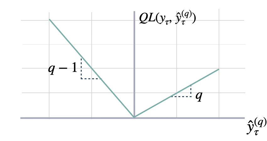
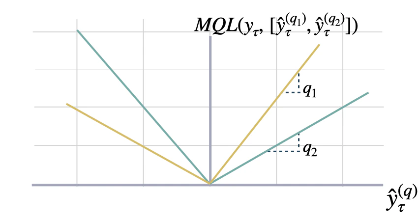
Computes the quantile loss between y and y_hat. QL measures the deviation of a quantile forecast. By weighting the absolute deviation in a non symmetric way, the loss pays more attention to under or over estimation. A common value for q is 0.5 for the deviation from the median (Pinball loss).

$$\mathrm{QL}(\mathbf{y}_{\tau}, \mathbf{\hat{y}}^{(q)}_{\tau}) = \frac{1}{H} \sum^{t+H}_{\tau=t+1} \Big( (1-q)\,( \hat{y}^{(q)}_{\tau} - y_{\tau} )_{+} + q\,( y_{\tau} - \hat{y}^{(q)}_{\tau} )_{+} \Big)$$

Parameters:

Name	Type	Description	Default
y	ndarray	Actual values.	required
y_hat	ndarray	Predicted values.	required
q	float	The slope of the quantile loss, in the context of quantile regression, the q determines the conditional quantile level. Defaults to 0.5.	0.5
mask	ndarray	Specifies date stamps per serie to consider in loss. Defaults to None.	required

Returns:

Name	Type	Description
float	Union[float, ndarray]	Quantile loss.

Multi-Quantile Loss

mqloss

mqloss(y, y_hat, quantiles, weights=None, axis=None)

Multi-Quantile loss

Calculates the Multi-Quantile loss (MQL) between y and y_hat. MQL calculates the average multi-quantile Loss for a given set of quantiles, based on the absolute difference between predicted quantiles and observed values.

$$\mathrm{MQL}(\mathbf{y}_{\tau},[\mathbf{\hat{y}}^{(q_{1})}_{\tau}, ... ,\hat{y}^{(q_{n})}_{\tau}]) = \frac{1}{n} \sum_{q_{i}} \mathrm{QL}(\mathbf{y}_{\tau}, \mathbf{\hat{y}}^{(q_{i})}_{\tau})$$

The limit behavior of MQL allows to measure the accuracy of a full predictive distribution $\\mathbf{\\hat{F}}\_{\\tau}$ with the continuous ranked probability score (CRPS). This can be achieved through a numerical integration technique, that discretizes the quantiles and treats the CRPS integral with a left Riemann approximation, averaging over uniformly distanced quantiles.

$$\mathrm{CRPS}(y_{\tau}, \mathbf{\hat{F}}_{\tau}) = \int^{1}_{0} \mathrm{QL}(y_{\tau}, \hat{y}^{(q)}_{\tau}) dq$$

Parameters:

Name	Type	Description	Default
y	ndarray	Actual values.	required
y_hat	ndarray	Predicted values.	required
quantiles	ndarray	Quantiles to estimate from the distribution of y.	required
mask	ndarray	Specifies date stamps per serie to consider in loss. Defaults to None.	required

Returns:

Name	Type	Description
float	Union[float, ndarray]	MQLoss.

James E. Matheson and Robert L. Winkler, “Scoring Rules for Continuous Probability Distributions”.

Examples and Validation

import unittest
import torch as t 
import numpy as np

from neuralforecast.losses.pytorch import (
    MAE, MSE, RMSE,      # unscaled errors
    MAPE, SMAPE,         # percentage errors
    MASE,                # scaled error
    QuantileLoss, MQLoss # probabilistic errors
)

from neuralforecast.losses.numpy import (
    mae, mse, rmse,              # unscaled errors
    mape, smape,                 # percentage errors
    mase,                        # scaled error
    quantile_loss, mqloss        # probabilistic errors
)