End to end walkthrough | MLForecast

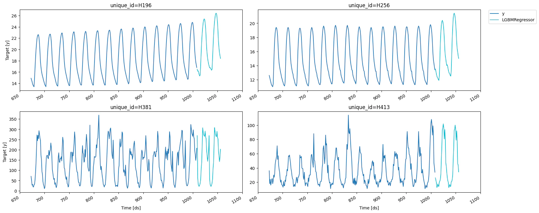
Detailed description of all the functionalities that MLForecast provides.

Data setup

For this example we’ll use a subset of the M4 hourly dataset. You can find the a notebook with the full dataset here.

import random
import tempfile
from pathlib import Path

import pandas as pd
from datasetsforecast.m4 import M4
from utilsforecast.plotting import plot_series

await M4.async_download('data', group='Hourly')
df, *_ = M4.load('data', 'Hourly')
uids = df['unique_id'].unique()
random.seed(0)
sample_uids = random.choices(uids, k=4)
df = df[df['unique_id'].isin(sample_uids)].reset_index(drop=True)
df['ds'] = df['ds'].astype('int64')
df

	unique_id	ds	y
0	H196	1	11.8
1	H196	2	11.4
2	H196	3	11.1
3	H196	4	10.8
4	H196	5	10.6
…	…	…	…
4027	H413	1004	99.0
4028	H413	1005	88.0
4029	H413	1006	47.0
4030	H413	1007	41.0
4031	H413	1008	34.0

EDA

We’ll take a look at our series to get ideas for transformations and features.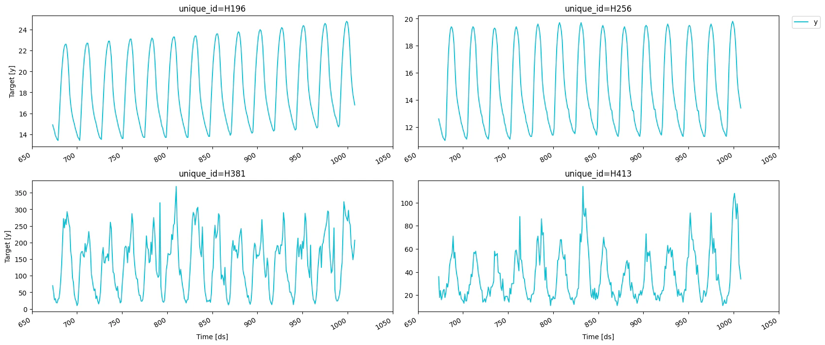

fig = plot_series(df, max_insample_length=24 * 14)

We can use the MLForecast.preprocess method to explore different transformations. It looks like these series have a strong seasonality on the hour of the day, so we can subtract the value from the same hour in the previous day to remove it. This can be done with the mlforecast.target_transforms.Differences transformer, which we pass through target_transforms.

from mlforecast import MLForecast
from mlforecast.target_transforms import Differences

fcst = MLForecast(
    models=[],  # we're not interested in modeling yet
    freq=1,  # our series have integer timestamps, so we'll just add 1 in every timestep
    target_transforms=[Differences([24])],
)
prep = fcst.preprocess(df)
prep

	unique_id	ds	y
24	H196	25	0.3
25	H196	26	0.3
26	H196	27	0.1
27	H196	28	0.2
28	H196	29	0.2
…	…	…	…
4027	H413	1004	39.0
4028	H413	1005	55.0
4029	H413	1006	14.0
4030	H413	1007	3.0
4031	H413	1008	4.0

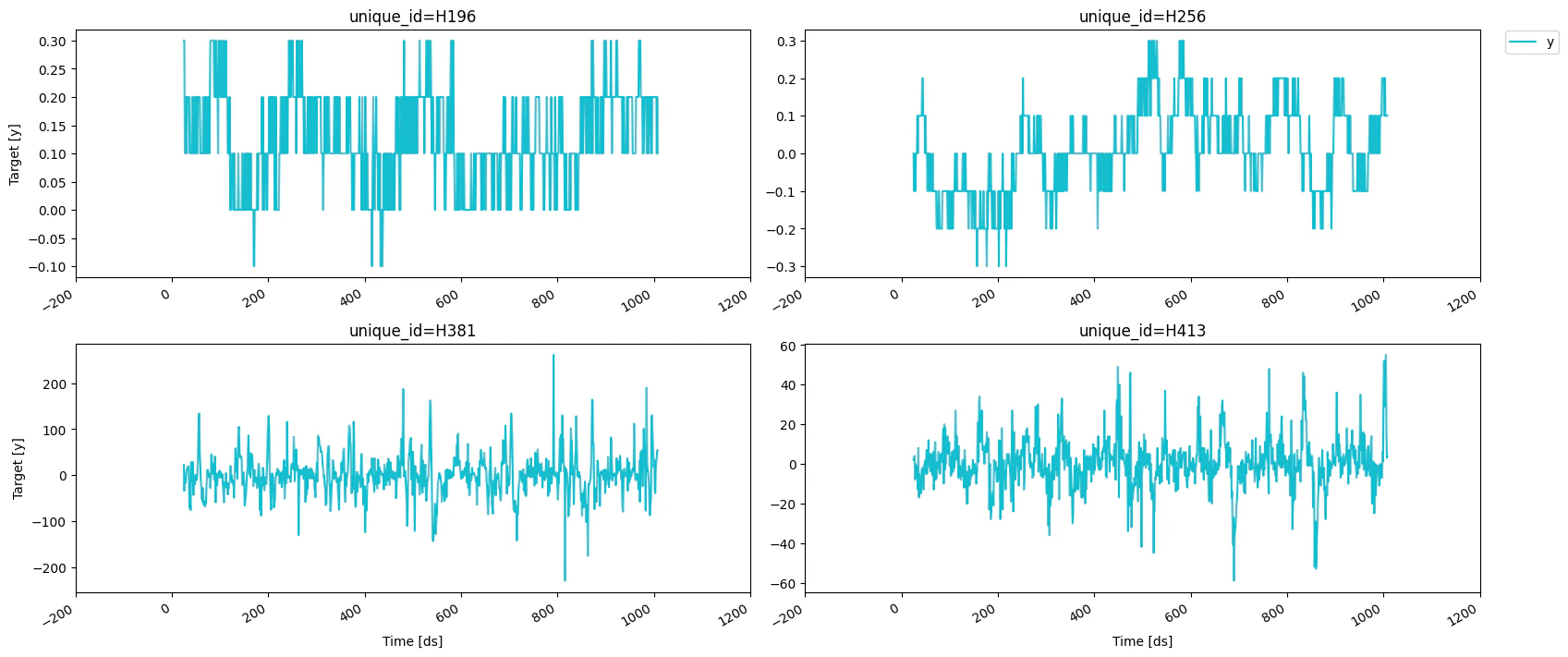
This has subtracted the lag 24 from each value, we can see what our series look like now.

fig = plot_series(prep)

Adding features

Lags

Looks like the seasonality is gone, we can now try adding some lag features.

fcst = MLForecast(
    models=[],
    freq=1,
    lags=[1, 24],
    target_transforms=[Differences([24])],    
)
prep = fcst.preprocess(df)
prep

	unique_id	ds	y	lag1	lag24
48	H196	49	0.1	0.1	0.3
49	H196	50	0.1	0.1	0.3
50	H196	51	0.2	0.1	0.1
51	H196	52	0.1	0.2	0.2
52	H196	53	0.1	0.1	0.2
…	…	…	…	…	…
4027	H413	1004	39.0	29.0	1.0
4028	H413	1005	55.0	39.0	-25.0
4029	H413	1006	14.0	55.0	-20.0
4030	H413	1007	3.0	14.0	0.0
4031	H413	1008	4.0	3.0	-16.0

prep.drop(columns=['unique_id', 'ds']).corr()['y']

y        1.000000
lag1     0.622531
lag24   -0.234268
Name: y, dtype: float64

Lag transforms

Lag transforms are defined as a dictionary where the keys are the lags and the values are the transformations that we want to apply to that lag. The lag transformations can be either objects from the mlforecast.lag_transforms module or numba jitted functions (so that computing the features doesn’t become a bottleneck and we can bypass the GIL when using multithreading), we have some implemented in the window-ops package but you can also implement your own.

from mlforecast.lag_transforms import ExpandingMean, RollingMean

from numba import njit
from window_ops.rolling import rolling_mean

@njit
def rolling_mean_48(x):
    return rolling_mean(x, window_size=48)


fcst = MLForecast(
    models=[],
    freq=1,
    target_transforms=[Differences([24])],    
    lag_transforms={
        1: [ExpandingMean()],
        24: [RollingMean(window_size=48), rolling_mean_48],
    },
)
prep = fcst.preprocess(df)
prep

	unique_id	ds	y	expanding_mean_lag1	rolling_mean_lag24_window_size48	rolling_mean_48_lag24
95	H196	96	0.1	0.174648	0.150000	0.150000
96	H196	97	0.3	0.173611	0.145833	0.145833
97	H196	98	0.3	0.175342	0.141667	0.141667
98	H196	99	0.3	0.177027	0.141667	0.141667
99	H196	100	0.3	0.178667	0.141667	0.141667
…	…	…	…	…	…	…
4027	H413	1004	39.0	0.242084	3.437500	3.437500
4028	H413	1005	55.0	0.281633	2.708333	2.708333
4029	H413	1006	14.0	0.337411	2.125000	2.125000
4030	H413	1007	3.0	0.351324	1.770833	1.770833
4031	H413	1008	4.0	0.354018	1.208333	1.208333

You can see that both approaches get to the same result, you can use whichever one you feel most comfortable with.

Date features

If your time column is made of timestamps then it might make sense to extract features like week, dayofweek, quarter, etc. You can do that by passing a list of strings with pandas time/date components. You can also pass functions that will take the time column as input, as we’ll show here.

def hour_index(times):
    return times % 24

fcst = MLForecast(
    models=[],
    freq=1,
    target_transforms=[Differences([24])],
    date_features=[hour_index],
)
fcst.preprocess(df)

	unique_id	ds	y	hour_index
24	H196	25	0.3	1
25	H196	26	0.3	2
26	H196	27	0.1	3
27	H196	28	0.2	4
28	H196	29	0.2	5
…	…	…	…	…
4027	H413	1004	39.0	20
4028	H413	1005	55.0	21
4029	H413	1006	14.0	22
4030	H413	1007	3.0	23
4031	H413	1008	4.0	0

Target transformations

If you want to do some transformation to your target before computing the features and then re-apply it after predicting you can use the target_transforms argument, which takes a list of transformations. You can find the implemented ones in mlforecast.target_transforms or you can implement your own as described in the target transformations guide.

from mlforecast.target_transforms import LocalStandardScaler

fcst = MLForecast(
    models=[],
    freq=1,
    lags=[1],
    target_transforms=[LocalStandardScaler()]
)
fcst.preprocess(df)

	unique_id	ds	y	lag1
1	H196	2	-1.493026	-1.383286
2	H196	3	-1.575331	-1.493026
3	H196	4	-1.657635	-1.575331
4	H196	5	-1.712505	-1.657635
5	H196	6	-1.794810	-1.712505
…	…	…	…	…
4027	H413	1004	3.062766	2.425012
4028	H413	1005	2.523128	3.062766
4029	H413	1006	0.511751	2.523128
4030	H413	1007	0.217403	0.511751
4031	H413	1008	-0.126003	0.217403

We can define a naive model to test this

from sklearn.base import BaseEstimator

class Naive(BaseEstimator):
    def fit(self, X, y):
        return self

    def predict(self, X):
        return X['lag1']

fcst = MLForecast(
    models=[Naive()],
    freq=1,
    lags=[1],
    target_transforms=[LocalStandardScaler()]
)
fcst.fit(df)
preds = fcst.predict(1)
preds

	unique_id	ds	Naive
0	H196	1009	16.8
1	H256	1009	13.4
2	H381	1009	207.0
3	H413	1009	34.0

We compare this with the last values of our series

last_vals = df.groupby('unique_id').tail(1)
last_vals

	unique_id	ds	y
1007	H196	1008	16.8
2015	H256	1008	13.4
3023	H381	1008	207.0
4031	H413	1008	34.0

import numpy as np

np.testing.assert_allclose(preds['Naive'], last_vals['y'])

Training

Once you’ve decided the features, transformations and models that you want to use you can use the MLForecast.fit method instead, which will do the preprocessing and then train the models. The models can be specified as a list (which will name them by using their class name and an index if there are repeated classes) or as a dictionary where the keys are the names you want to give to the models, i.e. the name of the column that will hold their predictions, and the values are the models themselves.

import lightgbm as lgb

lgb_params = {
    'verbosity': -1,
    'num_leaves': 512,
}

fcst = MLForecast(
    models={
        'avg': lgb.LGBMRegressor(**lgb_params),
        'q75': lgb.LGBMRegressor(**lgb_params, objective='quantile', alpha=0.75),
        'q25': lgb.LGBMRegressor(**lgb_params, objective='quantile', alpha=0.25),
    },
    freq=1,
    target_transforms=[Differences([24])],
    lags=[1, 24],
    lag_transforms={
        1: [ExpandingMean()],
        24: [RollingMean(window_size=48)],
    },
    date_features=[hour_index],
)
fcst.fit(df)

MLForecast(models=[avg, q75, q25], freq=1, lag_features=['lag1', 'lag24', 'expanding_mean_lag1', 'rolling_mean_lag24_window_size48'], date_features=[<function hour_index>], num_threads=1)

This computed the features and trained three different models using them. We can now compute our forecasts.

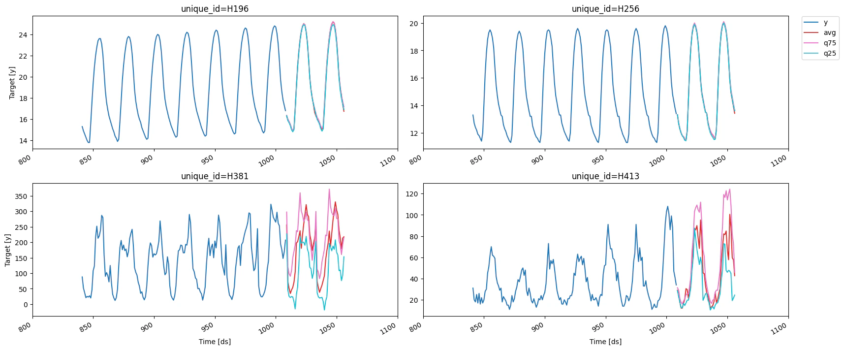
Forecasting

preds = fcst.predict(48)
preds

	unique_id	ds	avg	q75	q25
0	H196	1009	16.295257	16.357148	16.315731
1	H196	1010	15.910282	16.007322	15.862261
2	H196	1011	15.728367	15.780183	15.658180
3	H196	1012	15.468414	15.513598	15.399717
4	H196	1013	15.081279	15.133848	15.007694
…	…	…	…	…	…
187	H413	1052	100.450617	124.211150	47.025017
188	H413	1053	88.426800	108.303409	44.715380
189	H413	1054	59.675737	81.859964	19.239462
190	H413	1055	57.580356	72.703301	21.486674
191	H413	1056	42.669879	46.018271	24.392357

fig = plot_series(df, preds, max_insample_length=24 * 7)

Saving and loading

The MLForecast class has the MLForecast.save and MLForecast.load to store and then load the forecast object.

with tempfile.TemporaryDirectory() as tmpdir:
    save_dir = Path(tmpdir) / 'mlforecast'
    fcst.save(save_dir)
    fcst2 = MLForecast.load(save_dir)
    preds2 = fcst2.predict(48)
    pd.testing.assert_frame_equal(preds, preds2)

Updating series’ values

After you’ve trained a forecast object you can save and load it with the previous methods. If by the time you want to use it you already know the following values of the target you can use the MLForecast.update method to incorporate these, which will allow you to use these new values when computing predictions.

• If no new values are provided for a series that’s currently stored, only the previous ones are kept.
• If new series are included they are added to the existing ones.

fcst = MLForecast(
    models=[Naive()],
    freq=1,
    lags=[1, 2, 3],
)
fcst.fit(df)
fcst.predict(1)

	unique_id	ds	Naive
0	H196	1009	16.8
1	H256	1009	13.4
2	H381	1009	207.0
3	H413	1009	34.0

new_values = pd.DataFrame({
    'unique_id': ['H196', 'H256'],
    'ds': [1009, 1009],
    'y': [17.0, 14.0],
})
fcst.update(new_values)
preds = fcst.predict(1)
preds

	unique_id	ds	Naive
0	H196	1010	17.0
1	H256	1010	14.0
2	H381	1009	207.0
3	H413	1009	34.0

Estimating model performance

Cross validation

In order to get an estimate of how well our model will be when predicting future data we can perform cross validation, which consists of training a few models independently on different subsets of the data, using them to predict a validation set and measuring their performance.

Since our data depends on time, we make our splits by removing the last portions of the series and using them as validation sets. This process is implemented in MLForecast.cross_validation.

fcst = MLForecast(
    models=lgb.LGBMRegressor(**lgb_params),
    freq=1,
    target_transforms=[Differences([24])],
    lags=[1, 24],
    lag_transforms={
        1: [ExpandingMean()],
        24: [RollingMean(window_size=48)],
    },
    date_features=[hour_index],
)
cv_result = fcst.cross_validation(
    df,
    n_windows=4,  # number of models to train/splits to perform
    h=48,  # length of the validation set in each window
)
cv_result

	unique_id	ds	cutoff	y	LGBMRegressor
0	H196	817	816	15.3	15.383165
1	H196	818	816	14.9	14.923219
2	H196	819	816	14.6	14.667834
3	H196	820	816	14.2	14.275964
4	H196	821	816	13.9	13.973491
…	…	…	…	…	…
763	H413	1004	960	99.0	65.644823
764	H413	1005	960	88.0	71.717097
765	H413	1006	960	47.0	76.704377
766	H413	1007	960	41.0	53.446638
767	H413	1008	960	34.0	54.902634

fig = plot_series(forecasts_df=cv_result.drop(columns='cutoff'))

We can compute the RMSE on each split.

from utilsforecast.losses import rmse

def evaluate_cv(df):
    return rmse(df, models=['LGBMRegressor'], id_col='cutoff').set_index('cutoff')

split_rmse = evaluate_cv(cv_result)
split_rmse

	LGBMRegressor
cutoff
816	29.418172
864	34.257598
912	13.145763
960	35.066261

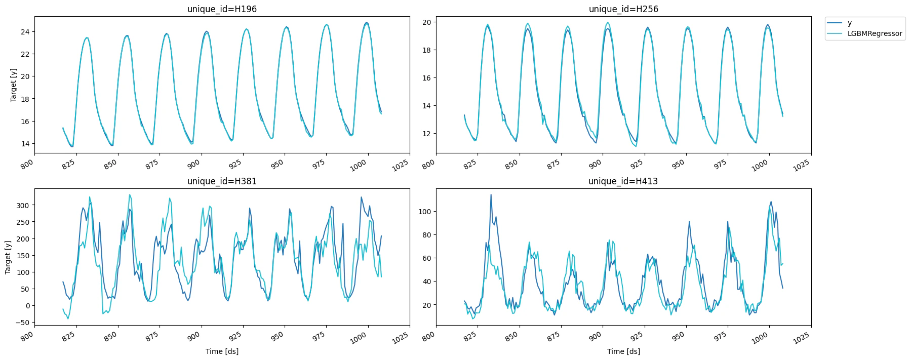
And the average RMSE across splits.

split_rmse.mean()

LGBMRegressor    27.971949
dtype: float64

You can quickly try different features and evaluate them this way. We can try removing the differencing and using an exponentially weighted average of the lag 1 instead of the expanding mean.

from mlforecast.lag_transforms import ExponentiallyWeightedMean

fcst = MLForecast(
    models=lgb.LGBMRegressor(**lgb_params),
    freq=1,
    lags=[1, 24],
    lag_transforms={
        1: [ExponentiallyWeightedMean(alpha=0.5)],
        24: [RollingMean(window_size=48)],      
    },
    date_features=[hour_index],    
)
cv_result2 = fcst.cross_validation(
    df,
    n_windows=4,
    h=48,
)
evaluate_cv(cv_result2).mean()

LGBMRegressor    25.874439
dtype: float64

LightGBMCV

In the same spirit of estimating our model’s performance, LightGBMCV allows us to train a few LightGBM models on different partitions of the data. The main differences with MLForecast.cross_validation are:

• It can only train LightGBM models.
• It trains all models simultaneously and gives us per-iteration averages of the errors across the complete forecasting window, which allows us to find the best iteration.

from mlforecast.lgb_cv import LightGBMCV

cv = LightGBMCV(
    freq=1,
    target_transforms=[Differences([24])],
    lags=[1, 24],
    lag_transforms={
        1: [ExpandingMean()],
        24: [RollingMean(window_size=48)],
    },
    date_features=[hour_index],
    num_threads=2,
)
cv_hist = cv.fit(
    df,
    n_windows=4,
    h=48,
    params=lgb_params,
    eval_every=5,
    early_stopping_evals=5,    
    compute_cv_preds=True,
)

[5] mape: 0.158639
[10] mape: 0.163739
[15] mape: 0.161535
[20] mape: 0.169491
[25] mape: 0.163690
[30] mape: 0.164198
Early stopping at round 30
Using best iteration: 5

As you can see this gives us the error by iteration (controlled by the eval_every argument) and performs early stopping (which can be configured with early_stopping_evals and early_stopping_pct). If you set compute_cv_preds=True the out-of-fold predictions are computed using the best iteration found and are saved in the cv_preds_ attribute.

cv.cv_preds_

	unique_id	ds	y	Booster	window
0	H196	817	15.3	15.473182	0
1	H196	818	14.9	15.038571	0
2	H196	819	14.6	14.849409	0
3	H196	820	14.2	14.448379	0
4	H196	821	13.9	14.148379	0
…	…	…	…	…	…
187	H413	1004	99.0	61.425396	3
188	H413	1005	88.0	62.886890	3
189	H413	1006	47.0	57.886890	3
190	H413	1007	41.0	38.849009	3
191	H413	1008	34.0	44.720562	3

fig = plot_series(forecasts_df=cv.cv_preds_.drop(columns='window'))

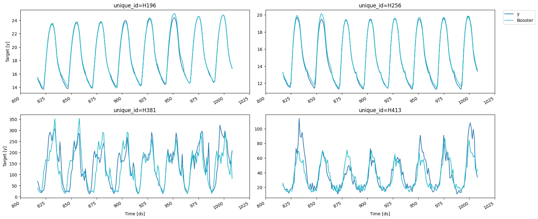
You can use this class to quickly try different configurations of features and hyperparameters. Once you’ve found a combination that works you can train a model with those features and hyperparameters on all the data by creating an MLForecast object from the LightGBMCV one as follows:

final_fcst = MLForecast.from_cv(cv)
final_fcst.fit(df)
preds = final_fcst.predict(48)
fig = plot_series(df, preds, max_insample_length=24 * 14)